Published: Dec 31, 2020 by Dev-hwon

이 내용은 고려대학교 강필성 교수님의 Business Analytics 수업을 보고 정리한 것입니다.

아래 이미지 클릭 시 강의 영상 Youtube URL로 넘어갑니다.

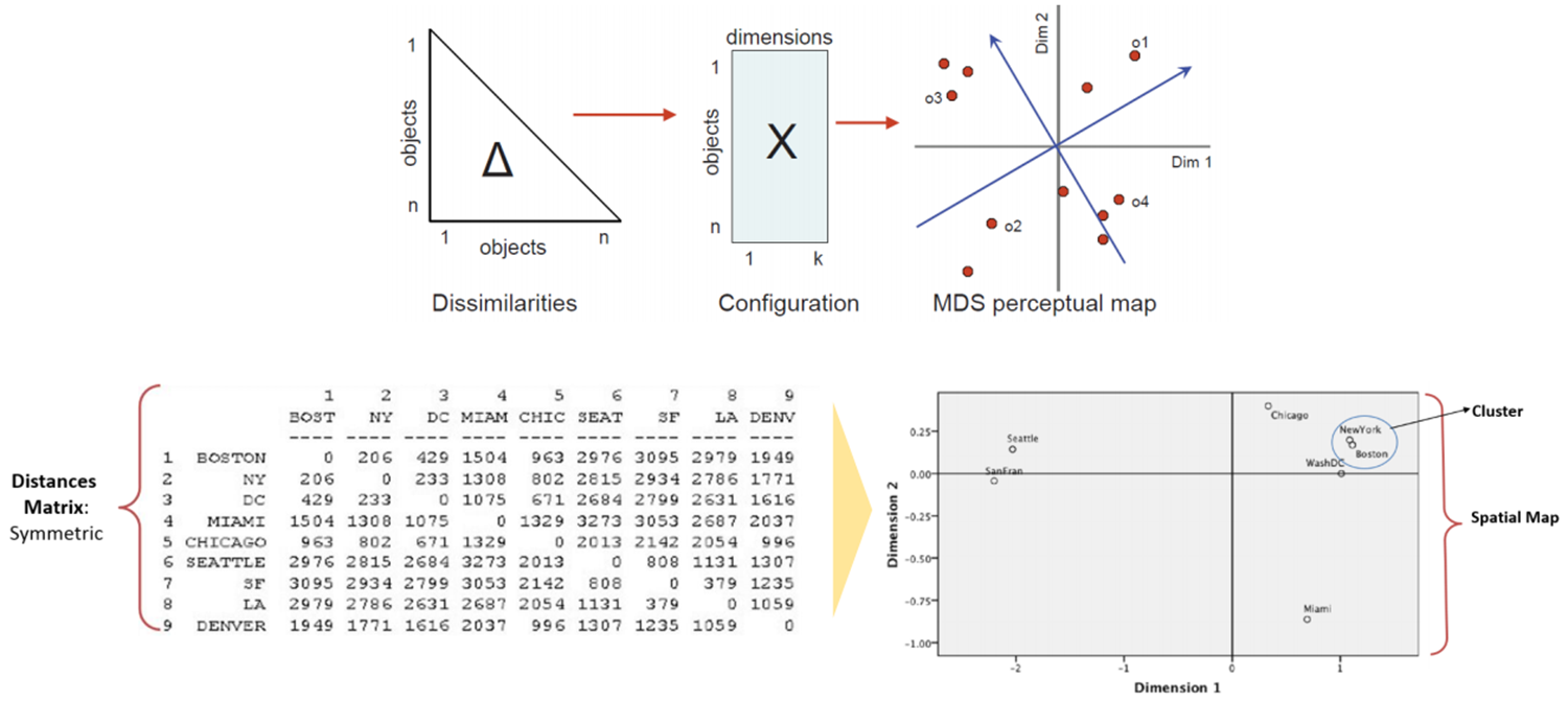
Multidimensional Scaling

• 객체들의 거리를 저차원 공간 상에서도 최대한 보존하는 것

PCA와 MDS 차이

	PCA	MDS
Data	d차원 공간의 n개 객체 (\(\textbf{X}\) in \(R^d\))	n 객체 사이의 근접 행렬 (n by n matrix \(\textbf{D}\))
Purpose	원래 분산을 최대한 유지하기 위한 기저셋 찾기	물체 간의 거리 정보를 유지하는 좌표 세트 찾기
Output	1. d bases (eigenvectors, PCs) 2. d eigenvalues	d 차원에서 각 개체의 좌표 (\(\textbf{X}\) in \(R^d\))

---

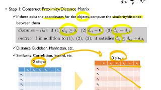
Step 1: Construct Proximity/Distance matrix

• 객체에 대한 좌표가 있으면 객체 간의 유사성/거리를 계산

\[distance-like \; \text{if} \; (1)\;d_{ij} \geq 0, \;(2)\;d_{ii}=0, \;(3)\; d_{ij}=d_{ji}\] \[metric\;\text{if in addition to (1), (2), (3), it satisfies }d_{ij}\leq d_{ik}+d_{jk}\]

• Distance: Euclidean, Manhattan, etc.
• Similarity: Correlation, Jaccard, etc. Distance, Similarity 보러가기

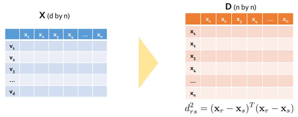
Step 2: Extract the coordinates that preserve the distance information

• 거리 행렬 D의 각 요소는 다음과 같이 표현할 수 있다.

\[d^2_{rs}=(\mathbf{x}_r-\mathbf{x}_s)^T(\mathbf{x}_r-\mathbf{x}_s)\]

• 내적 행렬 B는 거리 행렬 D에서 얻을 수 있다.

\[[\mathbf{B}]_{rs}=b_{rs}=\mathbf{x}^T_r\mathbf{x}_s\]

모든 p 변수의 평균이 0이라고 가정하면

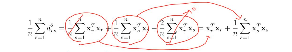
\[\sum^n_{r=1}x_{ri}=0, (i=1,2,\cdots,p) \;\;\;\;\;\;\;\;\; d^2_{rs}=\mathbf{x}^T_r\mathbf{x}_r+\mathbf{x}^T_s\mathbf{x}_s-2\mathbf{x}^T_r\mathbf{x}_s\]

• \(d^2_{rs}\)를 r에 대한 평균을 구하면 (여기서부터는 이해를 위해 계산되는 공식을 이미지로 대체 합니다.)

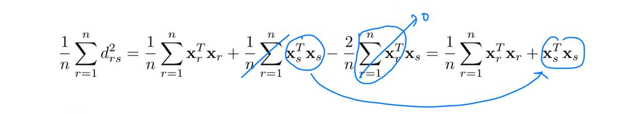
\(\frac{1}{n}\sum^n_{r=1}\mathbf{x}^T_r\mathbf{x}_r\)을 이항하면

\[\mathbf{x}^T_s\mathbf{x}_s=\frac{1}{n}\sum^n_{r=1}d^2_{rs}+\frac{1}{n}\sum^n_{r=1}\mathbf{x}^T_r\mathbf{x}_r\]

• \(d^2_{rs}\)를 s에 대한 평균을 구하면

\(\frac{1}{n}\sum^n_{r=1}\mathbf{x}^T_s\mathbf{x}_s\)을 이항하면

\[\mathbf{x}^T_r\mathbf{x}_r=\frac{1}{n}\sum^n_{r=1}d^2_{rs}+\frac{1}{n}\sum^n_{r=1}\mathbf{x}^T_s\mathbf{x}_s\]

• \(d^2_{rs}\)를 r과 s에 대한 평균을 구하면

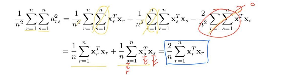
\(\frac{1}{n}\sum^n_{r=1}\mathbf{x}^T_s\mathbf{x}_s\)에서 \(s\)를 \(r\)로 바꿀 수 있다.(s는 임의의 수이기 때문)

\[\frac{2}{n}\sum^n_{r=1}\mathbf{x}^T_r\mathbf{x}_r=\frac{1}{n^2}\sum^n_{r=1}\sum^n_{s=1}d^2_{rs}\]

• \(b_{rs}\)를 구하면

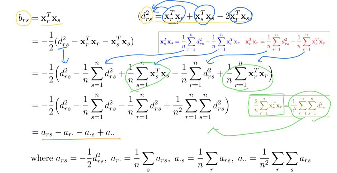
\([\mathbf{A}]_{rs}=a_{rs}\;\;\;\;\;\;\mathbf{B=HAH}\;\;\;\;\;\;\mathbf{H=I}-\frac{1}{n}\mathbf{11}^T\) 로 표현할 수 있다.

\(\mathbf{I}=\begin{pmatrix} 1 & \cdots & 0\\ \vdots & \ddots & \\ 0 & & 1 \end{pmatrix}\;\;\;\;\;\frac{1}{n}\mathbf{11}^T=\begin{pmatrix} \frac{1}{n} & \cdots & \frac{1}{n}\\ \vdots & \ddots & \\ \frac{1}{n} & & \frac{1}{n} \end{pmatrix}\)이다.

• B에서 X 좌표 구하기 (\(\mathbf{X} \text{: n by p, p <n}\))

\[\mathbf{B}=\mathbf{XX^T}\;\;\;\;rank(\mathbf{B})=rank(\mathbf{XX^T})=rank(\mathbf{X})=p\]

• B는 대칭이고 양의 준정부호 행렬이고 순위가 p이므로 음이 아닌 고유 값(eigenvalues)이 p 개이고 고유 값이 0이 n-p 개이다. (by Eigen-decomposition)

\[\mathbf{B}=\mathbf{V\Lambda V^T}, \;\;\;\; \mathbf{\Lambda}=diag(\lambda_1,\lambda_2,\cdots,\lambda_n), \;\;\mathbf{V}=[\mathbf{v_1, v_2, \cdots, v_n}]\]

\(\mathbf{\Lambda}\)는 eigenvalue들이 \(\mathbf{V}\)는 eigenvector들이 들어가 있다. \(\lambda_1\)이 가장 크고 \(\lambda_n\)이 가장 작다.

• 0인 고유 값 n-p개는 빼고 \(\mathbf{B}\)를 다시 쓰면

\[\mathbf{B_1}=\mathbf{V_1\Lambda_1 V_1^T}, \;\;\;\; \mathbf{\Lambda_1}=diag(\lambda_1,\lambda_2,\cdots,\lambda_p), \;\;\mathbf{V_1}=[\mathbf{v_1, v_2, \cdots, v_p}]\]

• \(\mathbf{B}=\mathbf{XX^T}\) 이므로 \(\mathbf{X}=\mathbf{V_1\Lambda_1^{\frac{1}{2}}}\)로 표현할 수 있다.

---

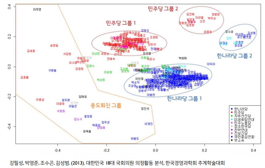
MDS 예제